Evaluate
Can seasonal forecasts be used as ‘alternate’ realities? Here we show how a set of evaluation metrics can be used to answer this question. The evaluation metrics are available through an R package for easy evaluation of the UNSEEN ensemble. Here, we illustrate how this package can be used in the UNSEEN workflow. We will evaluate the generated UNSEEN ensemble of UK February precipitation and of MAM Siberian heatwaves.
The framework to evaluate the UNSEEN ensemble presented here consists of testing the ensemble member independence, model stability and model fidelity, see also NPJ paper.
Note
This is R code and not python!
We switch to R since we believe R has a better functionality in extreme value statistics.
We load the UNSEEN package and read in the data.
[2]:
library(UNSEEN)
The data that is imported here are the files stored at the end of the preprocessing step.
[3]:
SEAS5_Siberia_events <- read.csv("Data/SEAS5_Siberia_events.csv", stringsAsFactors=FALSE)
ERA5_Siberia_events <- read.csv("Data/ERA5_Siberia_events.csv", stringsAsFactors=FALSE)
[4]:
SEAS5_Siberia_events_zoomed <- read.csv("Data/SEAS5_Siberia_events_zoomed.csv", stringsAsFactors=FALSE)
ERA5_Siberia_events_zoomed <- read.csv("Data/ERA5_Siberia_events_zoomed.csv", stringsAsFactors=FALSE)
[5]:
SEAS5_Siberia_events$t2m <- SEAS5_Siberia_events$t2m - 273.15
ERA5_Siberia_events$t2m <- ERA5_Siberia_events$t2m - 273.15
SEAS5_Siberia_events_zoomed$t2m <- SEAS5_Siberia_events_zoomed$t2m - 273.15
ERA5_Siberia_events_zoomed$t2m <- ERA5_Siberia_events_zoomed$t2m - 273.15
[6]:
head(SEAS5_Siberia_events_zoomed,n = 3)
head(ERA5_Siberia_events, n = 3)
| year | leadtime | number | t2m | |
|---|---|---|---|---|
| <int> | <int> | <int> | <dbl> | |
| 1 | 1982 | 2 | 0 | -3.736505 |
| 2 | 1982 | 2 | 1 | -5.682759 |
| 3 | 1982 | 2 | 2 | -4.221411 |
| year | t2m | |
|---|---|---|
| <int> | <dbl> | |
| 1 | 1979 | 4.010750 |
| 2 | 1980 | 3.880965 |
| 3 | 1981 | 4.822891 |
[7]:
EOBS_UK_weighted_df <- read.csv("Data/EOBS_UK_weighted_upscaled.csv", stringsAsFactors=FALSE)
SEAS5_UK_weighted_df <- read.csv("Data/SEAS5_UK_weighted_masked.csv", stringsAsFactors=FALSE)
And then convert the time class to Date format, with the ymd function in lubridate:
[8]:
EOBS_UK_weighted_df$time <- lubridate::ymd(EOBS_UK_weighted_df$time)
str(EOBS_UK_weighted_df)

EOBS_UK_weighted_df_hindcast <- EOBS_UK_weighted_df[
    EOBS_UK_weighted_df$time > '1982-02-01' &
    EOBS_UK_weighted_df$time < '2017-02-01',
    ]


SEAS5_UK_weighted_df$time <- lubridate::ymd(SEAS5_UK_weighted_df$time)
str(SEAS5_UK_weighted_df)
'data.frame':   71 obs. of  2 variables:
 $ time: Date, format: "1950-02-28" "1951-02-28" ...
 $ rr  : num  4.13 3.25 1.07 1.59 2.59 ...
'data.frame':   9945 obs. of  4 variables:
 $ leadtime: int  2 2 2 2 2 2 2 2 2 2 ...
 $ number  : int  0 0 0 0 0 0 0 0 0 0 ...
 $ time    : Date, format: "1982-02-01" "1983-02-01" ...
 $ tprate  : num  1.62 2.93 3.27 2 3.31 ...
Timeseries
Here we plot the timeseries of SEAS5 (UNSEEN) and ERA5 (OBS) for the Siberian Heatwave.
[10]:
unseen_timeseries(
    ensemble = SEAS5_Siberia_events_zoomed,
    obs = ERA5_Siberia_events_zoomed,
    ensemble_yname = "t2m",
    ensemble_xname = "year",
    obs_yname = "t2m",
    obs_xname = "year",
    ylab = "MAM Siberian temperature (C)")
Warning message:
“Removed 2756 rows containing non-finite values (stat_boxplot).”
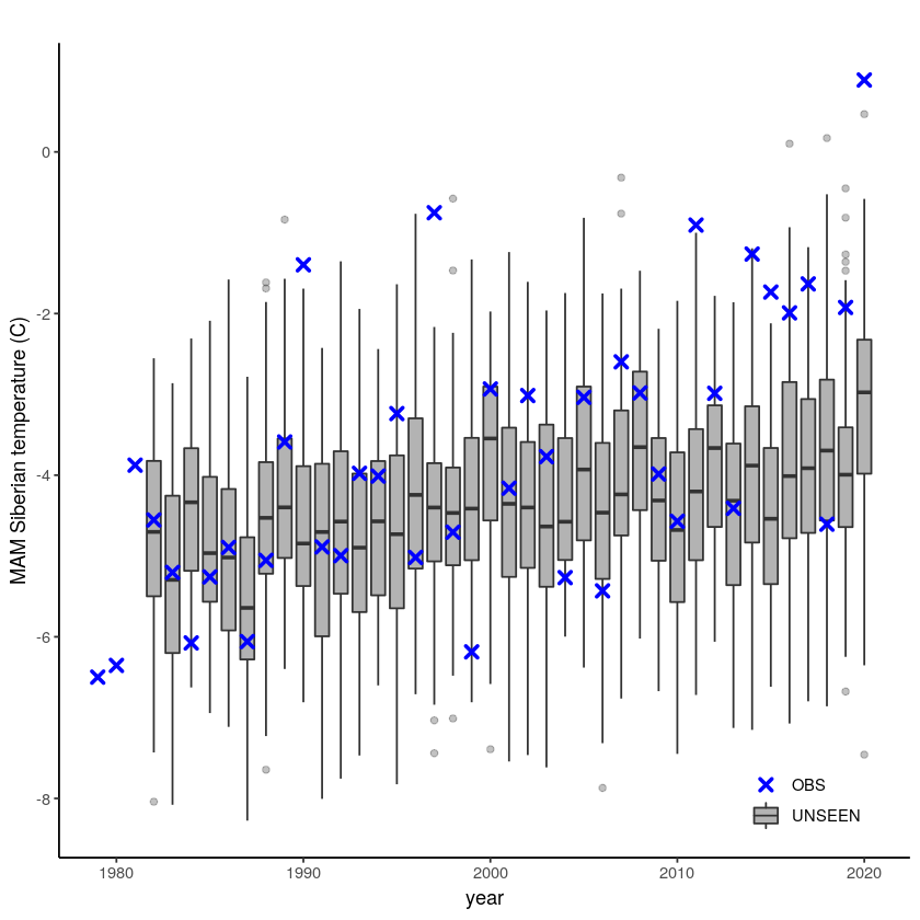
The timeseries consist of hindcast (years 1982-2016) and archived forecasts (years 2017-2020). The datasets are slightly different: the hindcasts contains 25 members whereas operational forecasts contain 51 members, the native resolution is different and the dataset from which the forecasts are initialized is different.
For the evaluation of the UNSEEN ensemble we want to only use the SEAS5 hindcasts for a consistent dataset. Note, 2017 is not used in either the hindcast nor the operational dataset in this example, since it contains forecasts both initialized in 2016 (hindcast) and 2017 (forecast), see retrieve. We split SEAS5 into hindcast and operational forecasts:
[11]:
SEAS5_Siberia_events_zoomed_hindcast <- SEAS5_Siberia_events_zoomed[
    SEAS5_Siberia_events_zoomed$year < 2017 &
    SEAS5_Siberia_events_zoomed$number < 25,]

SEAS5_Siberia_events_zoomed_forecasts <- SEAS5_Siberia_events_zoomed[
    SEAS5_Siberia_events_zoomed$year > 2017,]
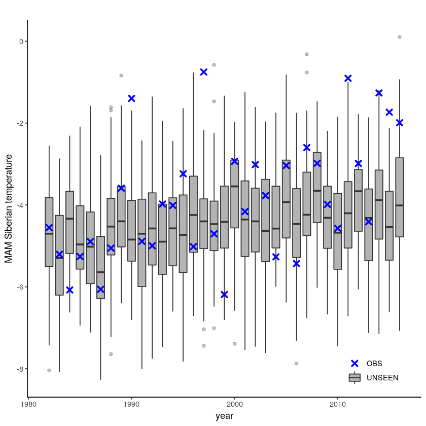
And we select the same years for ERA5.
[12]:
ERA5_Siberia_events_zoomed_hindcast <- ERA5_Siberia_events_zoomed[
    ERA5_Siberia_events_zoomed$year < 2017 &
    ERA5_Siberia_events_zoomed$year > 1981,]
[13]:
unseen_timeseries(
    ensemble = SEAS5_Siberia_events_zoomed_hindcast,
    obs = ERA5_Siberia_events_zoomed_hindcast,
    ensemble_yname = "t2m",
    ensemble_xname = "year",
    obs_yname = "t2m",
    obs_xname = "year",
    ylab = "MAM Siberian temperature")
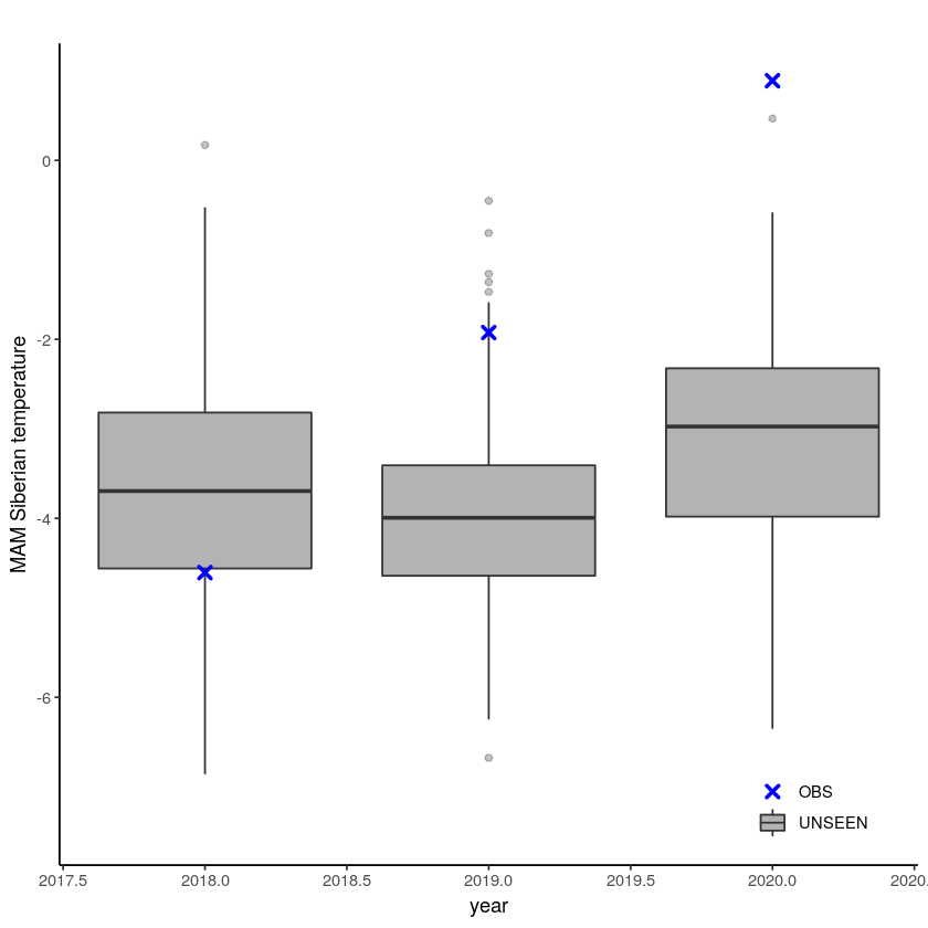
[14]:
unseen_timeseries(
    ensemble = SEAS5_Siberia_events_zoomed_forecasts,
    obs = ERA5_Siberia_events_zoomed[ERA5_Siberia_events_zoomed$year > 2017,],
    ensemble_yname = "t2m",
    ensemble_xname = "year",
    obs_yname = "t2m",
    obs_xname = "year",
    ylab = "MAM Siberian temperature")
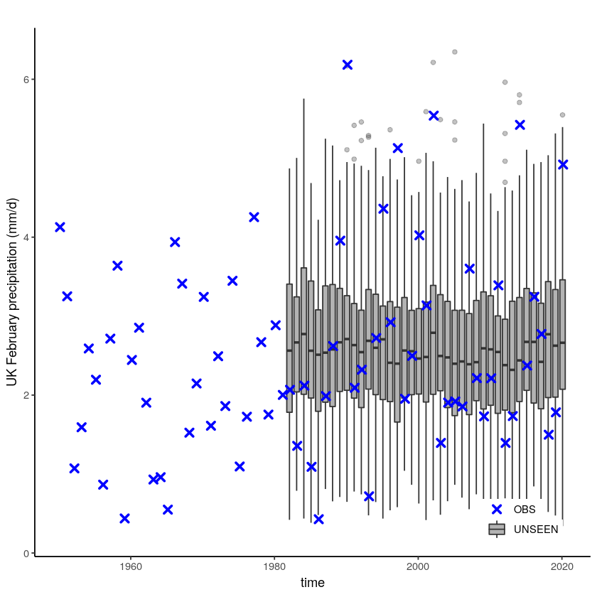
For the UK we have a longer historical record available from EOBS:
[15]:
unseen_timeseries(ensemble = SEAS5_UK_weighted_df,
                  obs = EOBS_UK_weighted_df,
                  ylab = 'UK February precipitation (mm/d)')
Warning message:
“Removed 4654 rows containing non-finite values (stat_boxplot).”
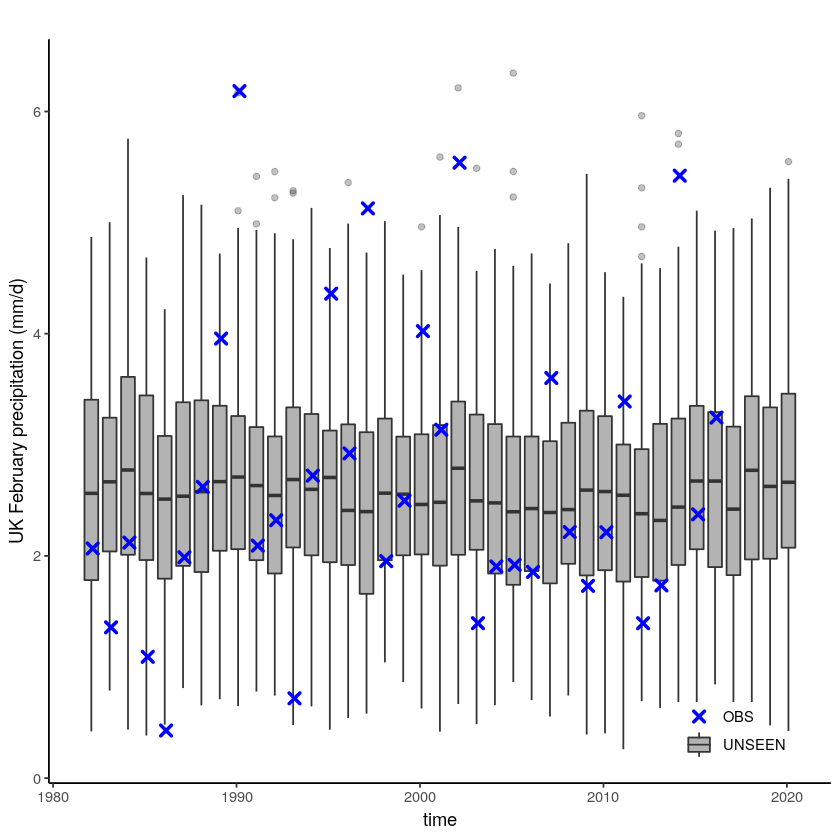
[16]:
unseen_timeseries(ensemble = SEAS5_UK_weighted_df,
                  obs = EOBS_UK_weighted_df_hindcast,
                  ylab = 'UK February precipitation (mm/d)')
Warning message:
“Removed 4654 rows containing non-finite values (stat_boxplot).”
Call the documentation of the function with ?unseen_timeseries
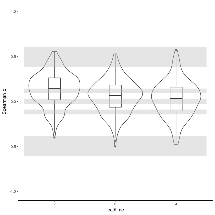
Independence
Significance ranges need fixing + detrend method (Rob)
[17]:
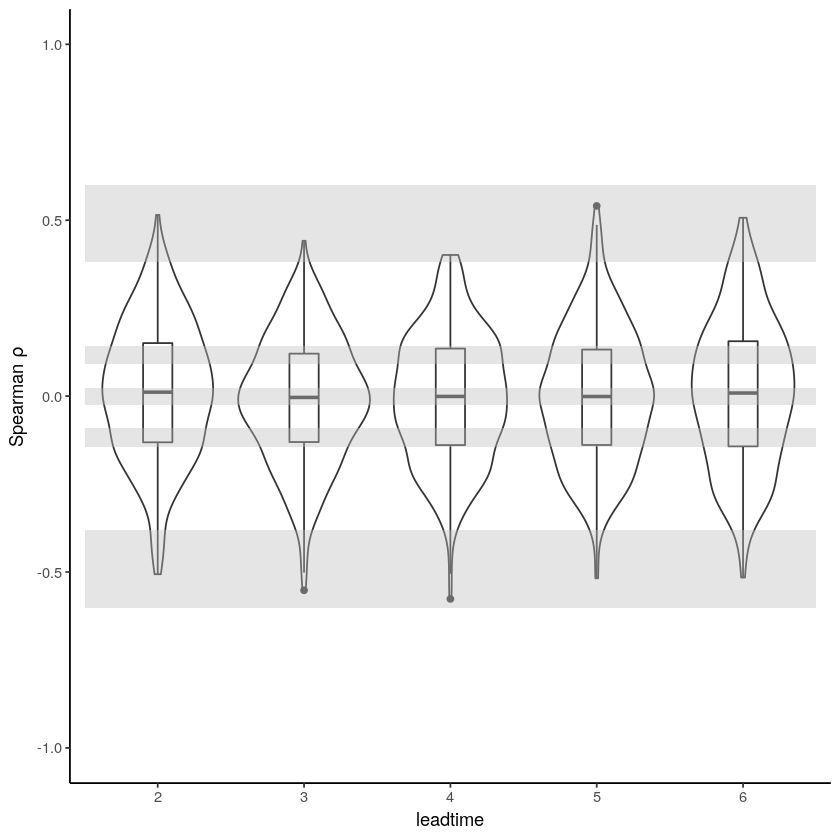
independence_test(
    ensemble = SEAS5_Siberia_events,
    n_lds = 3,
    var_name = "t2m",
)
Warning message:
“Removed 975 rows containing non-finite values (stat_ydensity).”
Warning message:
“Removed 975 rows containing non-finite values (stat_boxplot).”
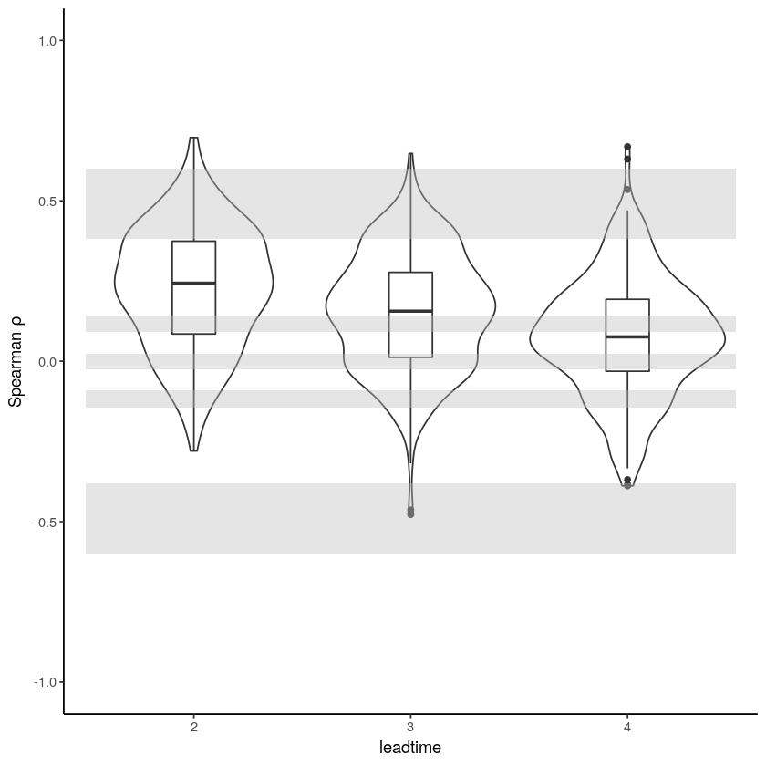
[18]:
independence_test(
    ensemble = SEAS5_Siberia_events_zoomed,
    n_lds = 3,
    var_name = "t2m",
)
Warning message:
“Removed 975 rows containing non-finite values (stat_ydensity).”
Warning message:
“Removed 975 rows containing non-finite values (stat_boxplot).”
[19]:
independence_test(ensemble = SEAS5_UK_weighted_df)
Warning message:
“Removed 1625 rows containing non-finite values (stat_ydensity).”
Warning message:
“Removed 1625 rows containing non-finite values (stat_boxplot).”
Stability
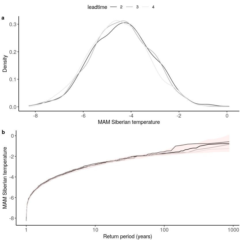
For the stability test we assess whether the events get more severe with leadtime, due to a potential ‘drift’ in the model. We need to use the consistent hindcast dataset for this.
[20]:
stability_test(
    ensemble = SEAS5_Siberia_events_zoomed_hindcast,
    lab = 'MAM Siberian temperature',
    var_name = 't2m'
)
Warning message:
“Removed 2 row(s) containing missing values (geom_path).”
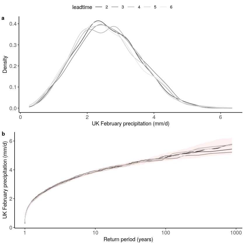
[21]:
stability_test(ensemble = SEAS5_UK, lab = 'UK February precipitation (mm/d)')
Warning message:
“Removed 4 row(s) containing missing values (geom_path).”
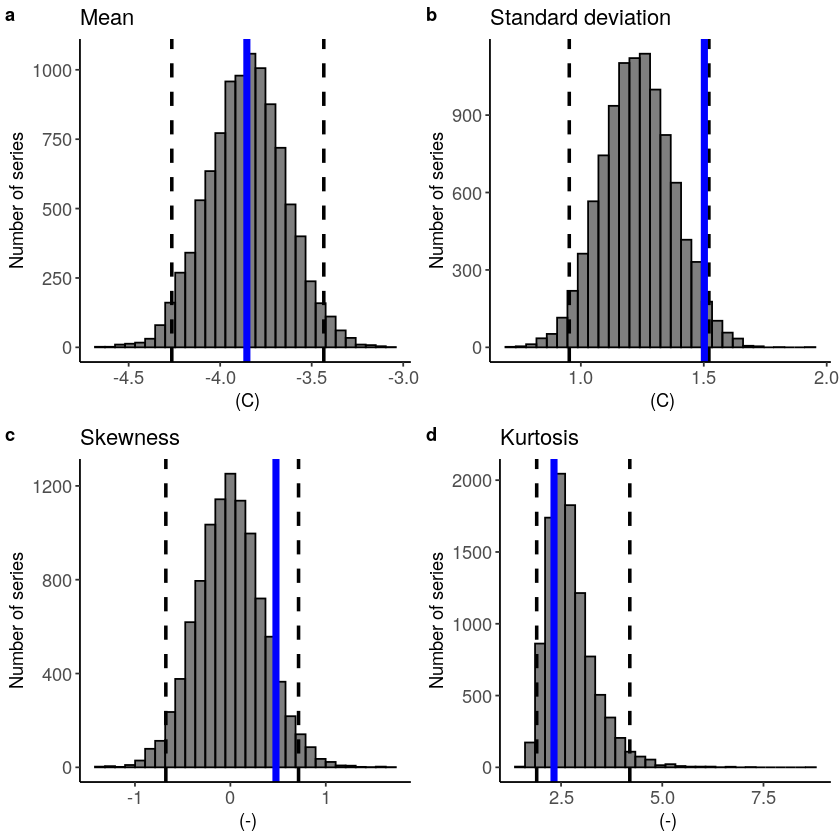
Fidelity
[22]:
fidelity_test(
    obs = ERA5_Siberia_events_zoomed_hindcast$t2m,
    ensemble = SEAS5_Siberia_events_zoomed_hindcast$t2m,
    units = 'C',
    biascor = FALSE
)
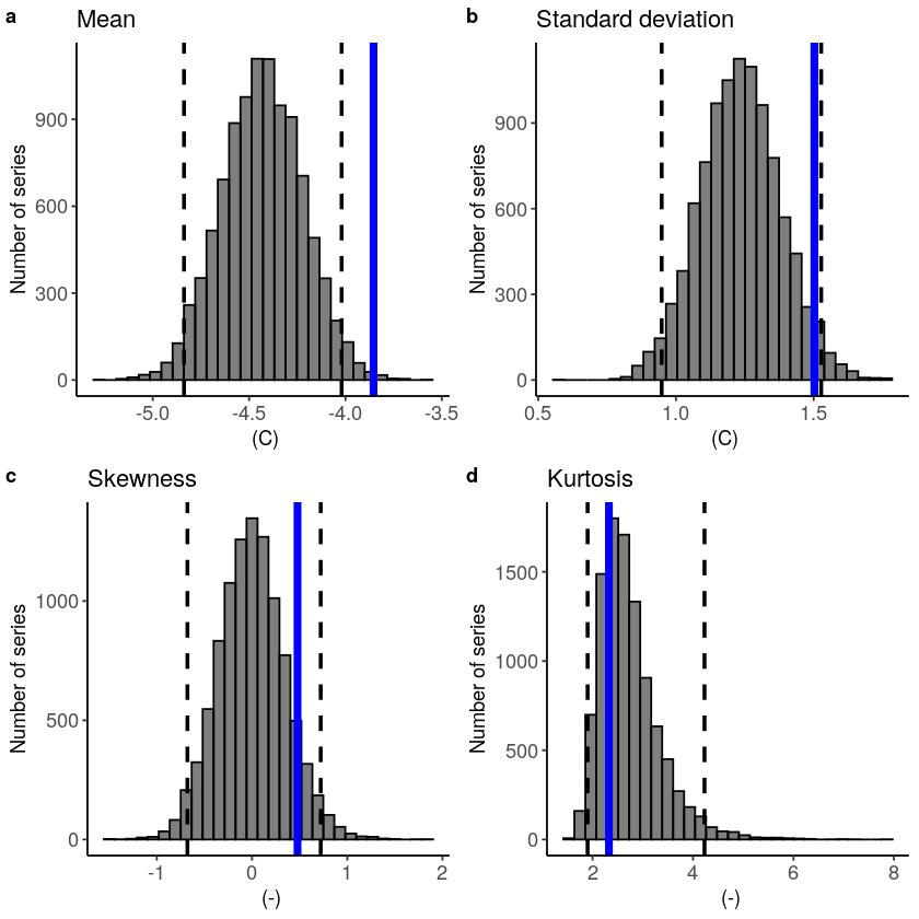
Lets apply a additive biascor
[23]:
#Lets apply a additive biascor
obs = ERA5_Siberia_events_zoomed_hindcast$t2m
ensemble = SEAS5_Siberia_events_zoomed_hindcast$t2m
ensemble_biascor = ensemble + (mean(obs) - mean(ensemble))

fidelity_test(
    obs = obs,
    ensemble = ensemble_biascor,
    units = 'C',
    biascor = FALSE
)